Prerequisite
For this exercise, we’ll need the campsismod package.
This package can be loaded as follows:
Create a minimalist model in the Notepad++ editor
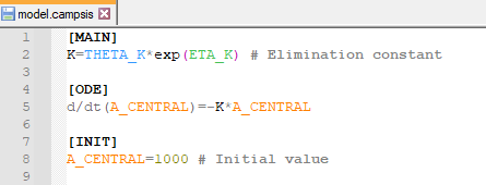
Assume a very simple 1-compartment PK model with first-order
eliminate rate K. Say this parameter has a typical value of
log(2)/12≈0.06 (where 12 is the elimination half life) and has 15% CV.
Let’s also initiate the central compartment to 1000.
This can be translated into the following Campsis model (
download Notepad++ plugin for Campsis):
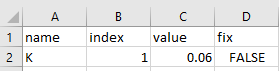
Let’s now create our theta.csv with our single parameter
K as follows:
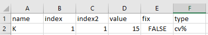
And finally, let’s also create our omega.csv to include
inter-individual variability on K:
This model can now be loaded by campsismod…
model <- read.campsis("resources/minimalist_model/")## Warning in read.allparameters(folder = folder): No file 'sigma.csv' could be
## found.Let’s simulated this model in Campsis:
library(campsis)
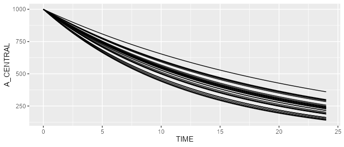
dataset <- Dataset(25) %>% add(Observations(seq(0,24,by=0.5)))
results <- model %>% simulate(dataset=dataset, seed=1)
spaghettiPlot(results, "A_CENTRAL")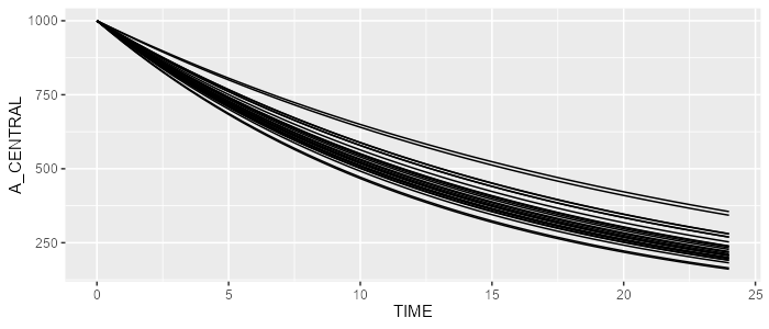
Create the same model programmatically
The same model can be created programmatically. First, let’s create an empty Campsis model.
model <- CampsisModel()Then, let’s define the equation of our model parameter
K.
We can add an ordinary differential equation as follows:
We can init the central compartment as well on the fly:
model <- model %>% add(InitialCondition(compartment=1, "1000"))Finally, let’s define our THETA_K and
ETA_K:
model <- model %>% add(Theta("K", value=0.06))
model <- model %>% add(Omega("K", value=15, type="cv%"))
This model can simulated by Campsis as well. Powerful, isn’t it?
library(campsis)
dataset <- Dataset(25) %>% add(Observations(seq(0,24,by=0.5)))
results <- model %>% simulate(dataset=dataset, seed=2)
spaghettiPlot(results, "A_CENTRAL")