Play with compartment properties
Source:vignettes/v04_compartment_properties.Rmd
v04_compartment_properties.RmdPrerequisite
For this vignette, please load the campsismod package
and load the minimalist model that we have created in the first
vignette.
library(campsismod)
model <- read.campsis("resources/minimalist_model/")
Create new compartment properties
Let’s invent a very basic scenario: we would like to infuse
1000 into the central compartment with a fixed rate of
100 and a fixed lag time of 2.
First, we’re going to delete the initial condition that we had in the
minimalist model. This is done as follows:
model_ <- model %>% delete(InitialCondition(compartment=1))
model_
## [MAIN]
## K=THETA_K*exp(ETA_K) # Elimination constant
##
## [ODE]
## d/dt(A_CENTRAL)=-K*A_CENTRAL
##
##
## THETA's:
## name index value fix
## 1 K 1 0.06 FALSE
## OMEGA's:
## name index index2 value fix type
## 1 K 1 1 15 FALSE cv%
## SIGMA's:
## # A tibble: 0 × 0
## No variance-covariance matrix
##
## Compartments:
## A_CENTRAL (CMT=1)This is strictly equal as doing (if you prefer working with compartment names):
model <- model %>% delete(InitialCondition(compartment= model %>% getCompartmentIndex("CENTRAL")))We can now add a fixed rate for all infusions that go into the central compartment:
model <- model %>% add(InfusionRate(compartment=1, "100"))Finally, let’s now add a constant lag time:
OK, this is how our model looks like now:
model## [MAIN]
## K=THETA_K*exp(ETA_K) # Elimination constant
##
## [ODE]
## d/dt(A_CENTRAL)=-K*A_CENTRAL
##
## [LAG]
## A_CENTRAL=2
##
## [RATE]
## A_CENTRAL=100
##
##
## THETA's:
## name index value fix
## 1 K 1 0.06 FALSE
## OMEGA's:
## name index index2 value fix type
## 1 K 1 1 15 FALSE cv%
## SIGMA's:
## # A tibble: 0 × 0
## No variance-covariance matrix
##
## Compartments:
## A_CENTRAL (CMT=1)Simulate our model
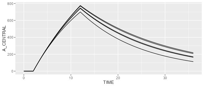
Let’s now simulate a few individuals and show A_CENTRAL,
i.e., the amount of drug in the central compartment.
First, we need to define an infusion of 1000 in a
Campsis dataset, as well as the observations times.
library(campsis)
dataset <- Dataset(5) %>%
  add(Infusion(time=0, amount=1000)) %>%
  add(Observations(seq(0,36,by=0.5)))
Then, we can run the simulation.
results <- model %>% simulate(dataset=dataset, seed=1)
spaghettiPlot(results, "A_CENTRAL")
A couple of useful functions in action
As previously, let’s demonstrate the use of a couple of interesting functions:
Check the existence of a compartment:
model %>% contains(Compartment(1)) ## [1] TRUE
# Or equivalenty:
model %>% contains(Compartment(model %>% getCompartmentIndex("CENTRAL")))
## [1] TRUECheck the existence of a property:
model %>% contains(InfusionRate(1))## [1] TRUE
model %>% contains(InfusionDuration(1)) ## [1] FALSEFind a compartment:
model %>% find(Compartment(1)) ## A_CENTRAL (CMT=1)Find a compartment property:
model %>% find(InfusionRate(1)) ## RATE (CMT=1): 100Replace a compartment property:
model %>% replace(InfusionRate(1, "200")) # Previous value of 100 is overridden## [MAIN]
## K=THETA_K*exp(ETA_K) # Elimination constant
##
## [ODE]
## d/dt(A_CENTRAL)=-K*A_CENTRAL
##
## [LAG]
## A_CENTRAL=2
##
## [RATE]
## A_CENTRAL=200
##
##
## THETA's:
## name index value fix
## 1 K 1 0.06 FALSE
## OMEGA's:
## name index index2 value fix type
## 1 K 1 1 15 FALSE cv%
## SIGMA's:
## # A tibble: 0 × 0
## No variance-covariance matrix
##
## Compartments:
## A_CENTRAL (CMT=1)Interestingly, the name of a compartment can be replaced as follows:
model %>% replace(Compartment(1, name="CENT")) %>%
  delete(Ode("A_CENTRAL")) %>%
  add(Ode("A_CENT", "-K*A_CENT"))
## [MAIN]
## K=THETA_K*exp(ETA_K) # Elimination constant
##
## [ODE]
## d/dt(A_CENT)=-K*A_CENT
##
## [LAG]
## A_CENT=2
##
## [RATE]
## A_CENT=100
##
##
## THETA's:
## name index value fix
## 1 K 1 0.06 FALSE
## OMEGA's:
## name index index2 value fix type
## 1 K 1 1 15 FALSE cv%
## SIGMA's:
## # A tibble: 0 × 0
## No variance-covariance matrix
##
## Compartments:
## A_CENT (CMT=1)