This vignette shows how a model can be appended to another. This is particularly useful when appending a PD model to a existing PK model. In this vignette, we’ll demonstrate how an effect compartment model can be appended to a 2-compartment model.
Load your base PK model
The following code will load our reference 2-compartment PK model.
pk_model <- model_suite$pk$`2cpt_fo`Load an effect-compartment model
The effect-compartment model can be loaded from the model library as follows:
pd_model <- model_suite$pd$effect_cmt_model
pd_model
## [MAIN]
## EMAX=THETA_EMAX*exp(ETA_EMAX)
## EC50=THETA_EC50*exp(ETA_EC50)
## GAMMA=THETA_GAMMA*exp(ETA_GAMMA)
## E0=THETA_E0*exp(ETA_E0)
## KE0=THETA_KE0*exp(ETA_KE0)
##
## [ODE]
## PK_CONC=10
## d/dt(A_ECONC)=KE0*(PK_CONC - A_ECONC)
## EFFECT=E0 + EMAX*pow(A_ECONC, GAMMA)/(pow(EC50, GAMMA) + pow(A_ECONC, GAMMA))
##
##
## THETA's:
## name index value fix label unit
## 1 EMAX 1 100.0 FALSE Maximum effect <NA>
## 2 EC50 2 10.0 FALSE Concentration at 50% of EMAX ng/mL
## 3 GAMMA 3 1.5 FALSE Hill coefficient <NA>
## 4 E0 4 20.0 FALSE Baseline <NA>
## 5 KE0 5 0.5 FALSE Effect compartment delay rate 1/h
## OMEGA's:
## name index index2 value fix type
## 1 EMAX 1 1 10 FALSE cv%
## 2 EC50 2 2 10 FALSE cv%
## 3 GAMMA 3 3 10 FALSE cv%
## 4 E0 4 4 10 FALSE cv%
## 5 KE0 5 5 10 FALSE cv%
## SIGMA's:
## # A tibble: 0 × 0
## No variance-covariance matrix
##
## Compartments:
## A_ECONC (CMT=1)This PD model has a variable PK_CONC, that needs to be
linked with the PK concentration.
Therefore, we need to adapt it as follows:
Append PD model to PK model
Appending the PD model to the PK model is done using the
add function:
## [MAIN]
## TVBIO=THETA_BIO
## TVKA=THETA_KA
## TVVC=THETA_VC
## TVVP=THETA_VP
## TVQ=THETA_Q
## TVCL=THETA_CL
##
## BIO=TVBIO
## KA=TVKA * exp(ETA_KA)
## VC=TVVC * exp(ETA_VC)
## VP=TVVP * exp(ETA_VP)
## Q=TVQ * exp(ETA_Q)
## CL=TVCL * exp(ETA_CL)
## EMAX=THETA_EMAX*exp(ETA_EMAX)
## EC50=THETA_EC50*exp(ETA_EC50)
## GAMMA=THETA_GAMMA*exp(ETA_GAMMA)
## E0=THETA_E0*exp(ETA_E0)
## KE0=THETA_KE0*exp(ETA_KE0)
##
## [ODE]
## d/dt(A_ABS)=-KA*A_ABS
## d/dt(A_CENTRAL)=KA*A_ABS + Q/VP*A_PERIPHERAL - Q/VC*A_CENTRAL - CL/VC*A_CENTRAL
## d/dt(A_PERIPHERAL)=Q/VC*A_CENTRAL - Q/VP*A_PERIPHERAL
## PK_CONC=A_CENTRAL/VC
## d/dt(A_ECONC)=KE0*(PK_CONC - A_ECONC)
## EFFECT=E0 + EMAX*pow(A_ECONC, GAMMA)/(pow(EC50, GAMMA) + pow(A_ECONC, GAMMA))
##
## [F]
## A_ABS=BIO
##
## [ERROR]
## CONC=A_CENTRAL/VC
## if (CONC <= 0.001) CONC=0.001
## CONC_ERR=CONC*(1 + EPS_PROP_RUV)
##
##
## THETA's:
##     name index value   fix                            label  unit
## 1    BIO     1   1.0 FALSE                  Bioavailability  <NA>
## 2     KA     2   1.0 FALSE                  Absorption rate   1/h
## 3     VC     3  10.0 FALSE    Volume of central compartment     L
## 4     VP     4  40.0 FALSE Volume of peripheral compartment     L
## 5      Q     5  20.0 FALSE           Inter-compartment flow   L/h
## 6     CL     6   3.0 FALSE                        Clearance   L/h
## 7   EMAX     7 100.0 FALSE                   Maximum effect  <NA>
## 8   EC50     8  10.0 FALSE     Concentration at 50% of EMAX ng/mL
## 9  GAMMA     9   1.5 FALSE                 Hill coefficient  <NA>
## 10    E0    10  20.0 FALSE                         Baseline  <NA>
## 11   KE0    11   0.5 FALSE    Effect compartment delay rate   1/h
## OMEGA's:
##     name index index2 value   fix type
## 1     KA     1      1    25 FALSE  cv%
## 2     VC     2      2    25 FALSE  cv%
## 3     VP     3      3    25 FALSE  cv%
## 4      Q     4      4    25 FALSE  cv%
## 5     CL     5      5    25 FALSE  cv%
## 6   EMAX     6      6    10 FALSE  cv%
## 7   EC50     7      7    10 FALSE  cv%
## 8  GAMMA     8      8    10 FALSE  cv%
## 9     E0     9      9    10 FALSE  cv%
## 10   KE0    10     10    10 FALSE  cv%
## SIGMA's:
##       name index index2 value   fix type
## 1 PROP_RUV     1      1   0.1 FALSE   sd
## No variance-covariance matrix
##
## Compartments:
## A_ABS (CMT=1)
## A_CENTRAL (CMT=2)
## A_PERIPHERAL (CMT=3)
## A_ECONC (CMT=4)
Simulate our PK/PD model
Let’s now simulate our PK/PD model:
library(campsis)
dataset <- Dataset(25) %>%
  add(Bolus(time=0, amount=1000, compartment=1, ii=12, addl=2)) %>%
  add(Observations(times=0:36))
results <- pkpd_model %>% simulate(dataset=dataset, seed=1)
shadedPlot(results, "CONC")
shadedPlot(results, "CONC")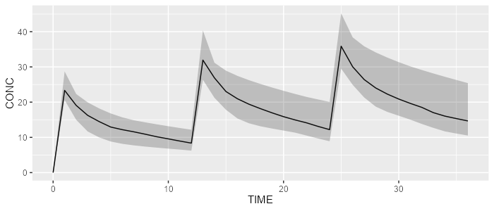
PK concentration
shadedPlot(results, "EFFECT")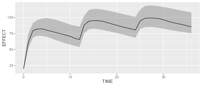
Showing the delayed effect