Simulate with all variabilities
Let’s use a simple 1-compartment model with absorption compartment to illustrate the different levels of variabilities.
ref_model <- model_suite$nonmem$advan2_trans2
ref_model
## [MAIN]
## KA=THETA_KA*exp(ETA_KA)
## CL=THETA_CL*exp(ETA_CL)
## V=THETA_V*exp(ETA_V)
## S2=V
##
## [ODE]
## d/dt(A_DEPOT)=-KA*A_DEPOT
## d/dt(A_CENTRAL)=-CL*A_CENTRAL/V + KA*A_DEPOT
## d/dt(A_OUTPUT)=CL*A_CENTRAL/V
## F=A_CENTRAL/S2
##
## [ERROR]
## CONC=F
## CONC_ERR=CONC*(EPS_PROP + 1)
##
##
## THETA's:
## name index value fix
## 1 KA 1 1 FALSE
## 2 CL 2 5 FALSE
## 3 V 3 80 FALSE
## OMEGA's:
## name index index2 value fix type
## 1 KA 1 1 0.025 FALSE var
## 2 CL 2 2 0.025 FALSE var
## 3 V 3 3 0.025 FALSE var
## SIGMA's:
## name index index2 value fix type
## 1 PROP 1 1 0.025 FALSE var
## No variance-covariance matrix
##
## Compartments:
## A_DEPOT (CMT=1)
## A_CENTRAL (CMT=2)
## A_OUTPUT (CMT=3)We’re going to use a very basic dataset. 1000 mg QD shall be administered for a week.
ds <- Dataset(25) %>%
  add(Bolus(time = 0, amount = 1000, ii = 24, addl = 6)) %>%
  add(Observations(times = seq(0, 24 * 7, by = 4)))
All subjects are different due to IIV and RUV.
results <- simulate(model = ref_model, dataset = ds, seed = 1)
spaghetti_plot(results, "CONC_ERR")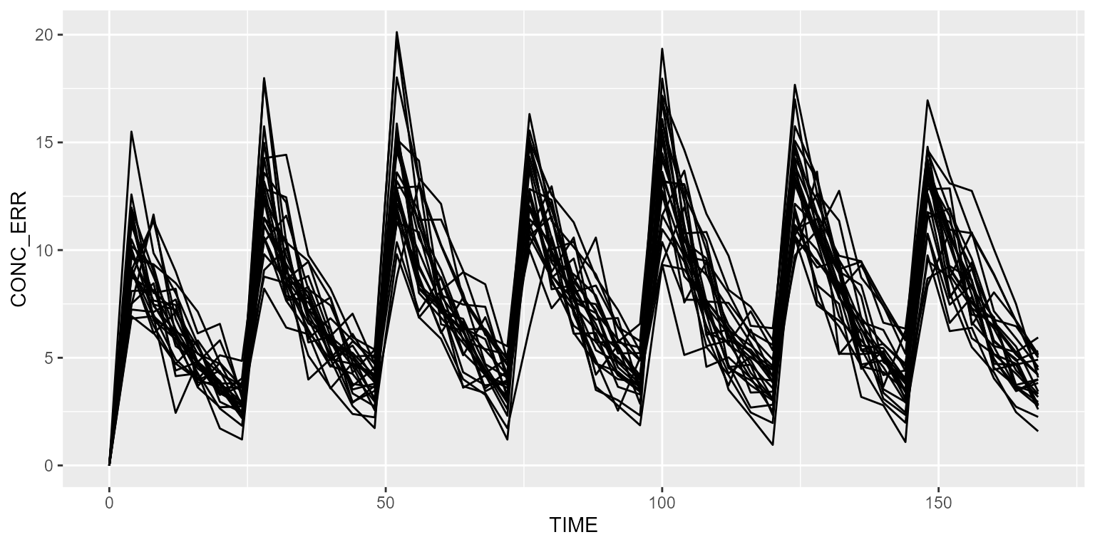
Simulate without RUV
Disabling RUV is done as follows:
## THETA's:
##   name index value   fix
## 1   KA     1     1 FALSE
## 2   CL     2     5 FALSE
## 3    V     3    80 FALSE
## OMEGA's:
##   name index index2 value   fix type
## 1   KA     1      1 0.025 FALSE  var
## 2   CL     2      2 0.025 FALSE  var
## 3    V     3      3 0.025 FALSE  var
## SIGMA's:
##   name index index2 value   fix type
## 1 PROP     1      1     0 FALSE  var
## No variance-covariance matrix
In that case, CONC_ERR (the observed concentration) is identical as CONC (the model-simulated plasma concentration).
results <- simulate(model = model, dataset = ds, seed = 1)
spaghetti_plot(results, "CONC_ERR")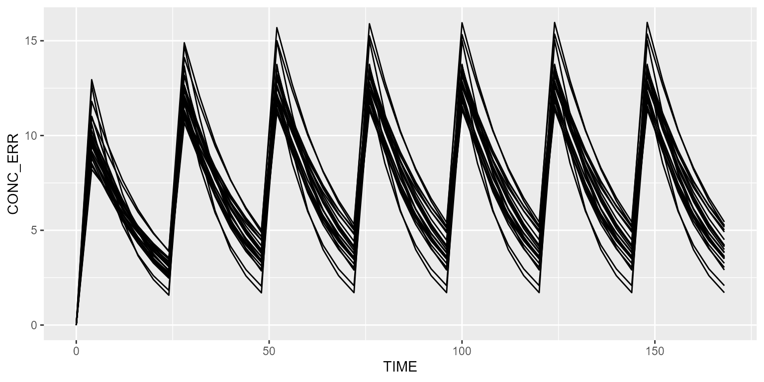
spaghetti_plot(results, "CONC")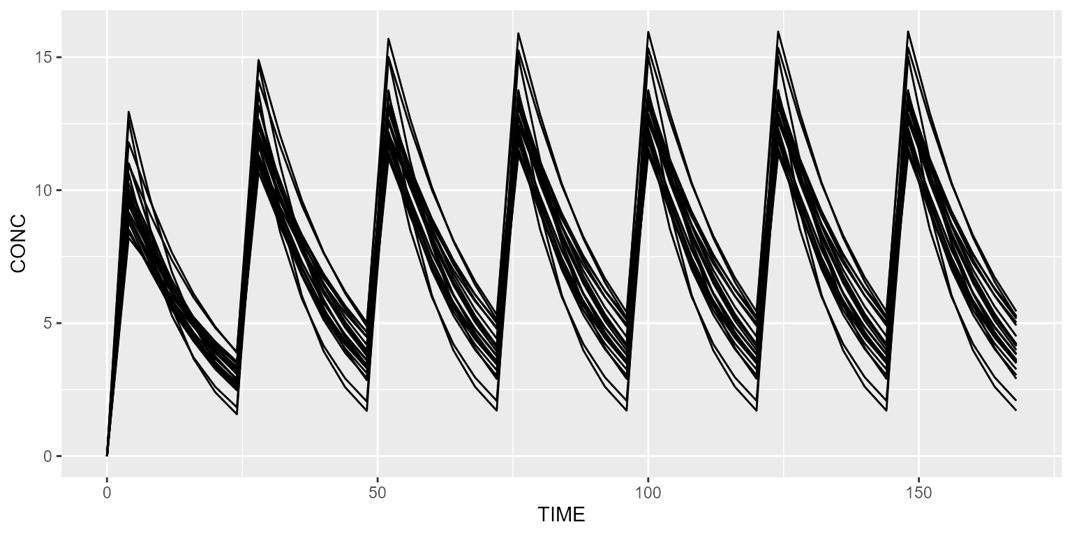
Simulate without RUV and IIV
Disabling RUV and IIV is done as follows:
## THETA's:
##   name index value   fix
## 1   KA     1     1 FALSE
## 2   CL     2     5 FALSE
## 3    V     3    80 FALSE
## OMEGA's:
##   name index index2 value   fix type
## 1   KA     1      1     0 FALSE  var
## 2   CL     2      2     0 FALSE  var
## 3    V     3      3     0 FALSE  var
## SIGMA's:
##   name index index2 value   fix type
## 1 PROP     1      1     0 FALSE  var
## No variance-covariance matrix
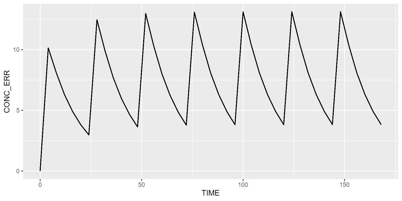
Now, the typical profile is shown for all subjects.
results <- model %>%
  simulate(dataset = ds, seed = 1)
spaghetti_plot(results, "CONC_ERR")