Add a body weight covariate into the model
Let’s use a simple 1-compartment model to illustrate how covariates are managed by CAMPSIS.
model <- model_suite$nonmem$advan1_trans2For this example, we’re going to add allometric scaling on the clearance parameter.
## [MAIN]
## CL=THETA_CL*exp(ETA_CL)*pow(BW/70, 0.75)
## V=THETA_V*exp(ETA_V)
## S1=V
##
## [ODE]
## d/dt(A_CENTRAL)=-CL*A_CENTRAL/V
## d/dt(A_OUTPUT)=CL*A_CENTRAL/V
## F=A_CENTRAL/S1
##
## [ERROR]
## CONC=F
## CONC_ERR=CONC*(EPS_PROP + 1)
##
##
## THETA's:
##   name index value   fix
## 1   CL     1     5 FALSE
## 2    V     2    80 FALSE
## OMEGA's:
##   name index index2 value   fix type
## 1   CL     1      1 0.025 FALSE  var
## 2    V     2      2 0.025 FALSE  var
## SIGMA's:
##   name index index2 value   fix type
## 1 PROP     1      1 0.025 FALSE  var
## No variance-covariance matrix
##
## Compartments:
## A_CENTRAL (CMT=1)
## A_OUTPUT (CMT=2)
We will infuse 1000 mg with a rate of 200 mg/hour into the central compartment and observe for a day. The corresponding dataset is as follows:
dataset <- Dataset() %>%
    add(Infusion(time=0, amount=1000, rate=200)) %>%
    add(Observations(times=seq(0,24,by=0.5)))
To visualize clearly the effect of the covariates, we will disable the inter-individual variability on the model.
Constant body weight
Let’s define a constant covariate into the dataset. This is done as follows.
ds <- dataset %>% setSubjects(5) %>%
  add(Covariate("BW", 70))
All simulated subjects will be exactly the same, as IIV was removed.
results <- model %>% simulate(dataset=ds)
spaghettiPlot(results, "CONC")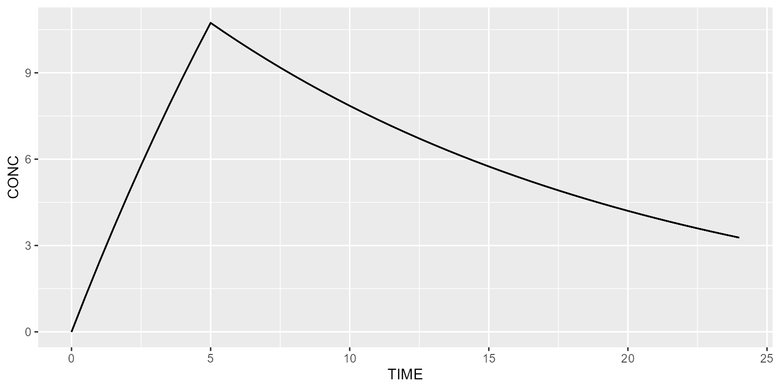
Fix body weight values (1/subject)
Let’s now define 1 body weight per subject. This is done as follows.
Simulated subjects should now be different.
results <- model %>% simulate(dataset=ds)
spaghettiPlot(results, "CONC")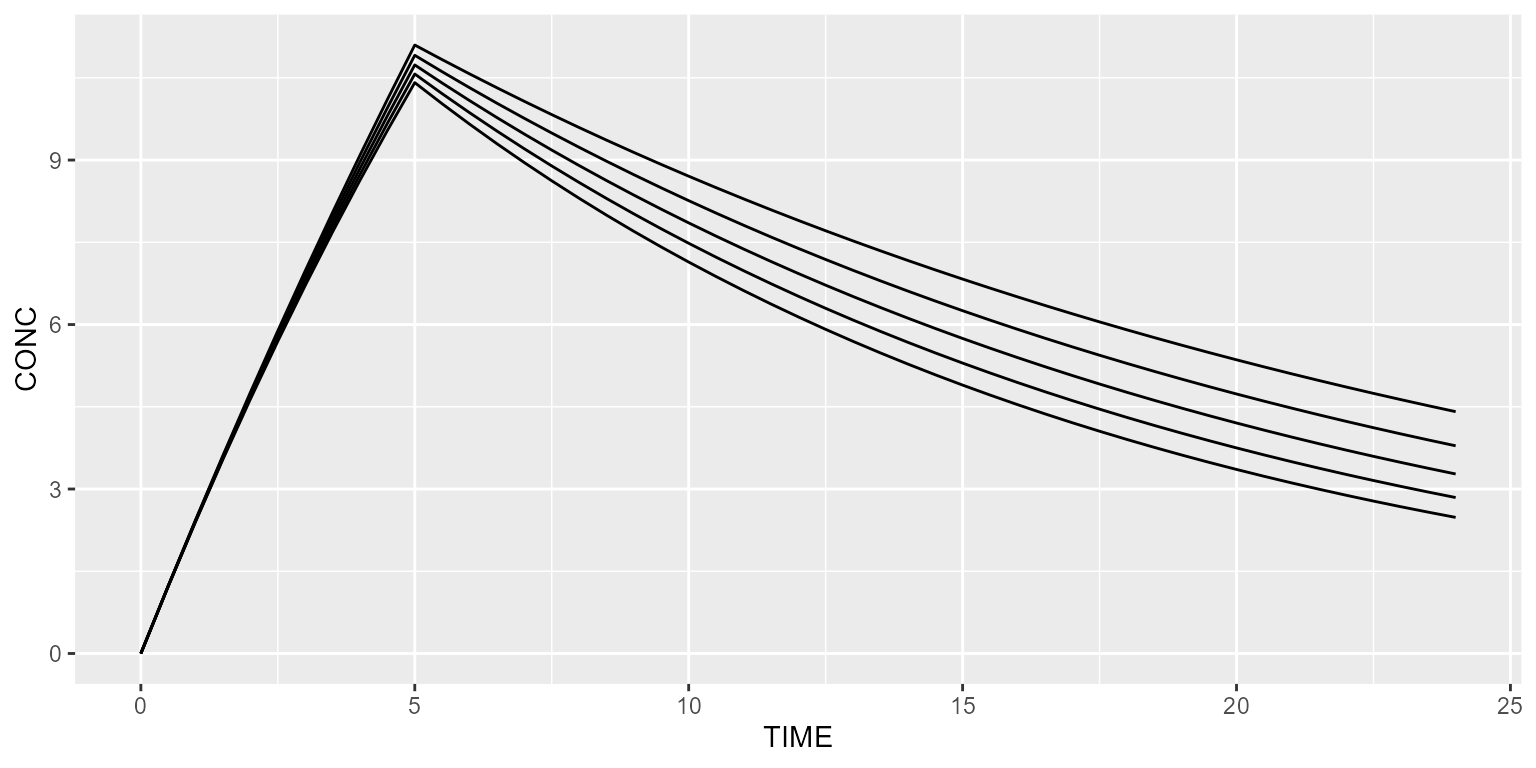
Uniform distribution
Let’s say now that the body weight is a uniform distribution. This can be implemented as follows:
ds <- dataset %>% setSubjects(40) %>%
  add(Covariate("BW", UniformDistribution(min=50, max=90)))
Simulated weights will then be sampled from a uniform distribution with a min value of 50 and a max value of 90.
results <- model %>% simulate(dataset=ds, outvars=c("CONC", "BW"), seed=1)
gridExtra::grid.arrange(spaghettiPlot(results, "BW"), spaghettiPlot(results, "CONC"), nrow=1)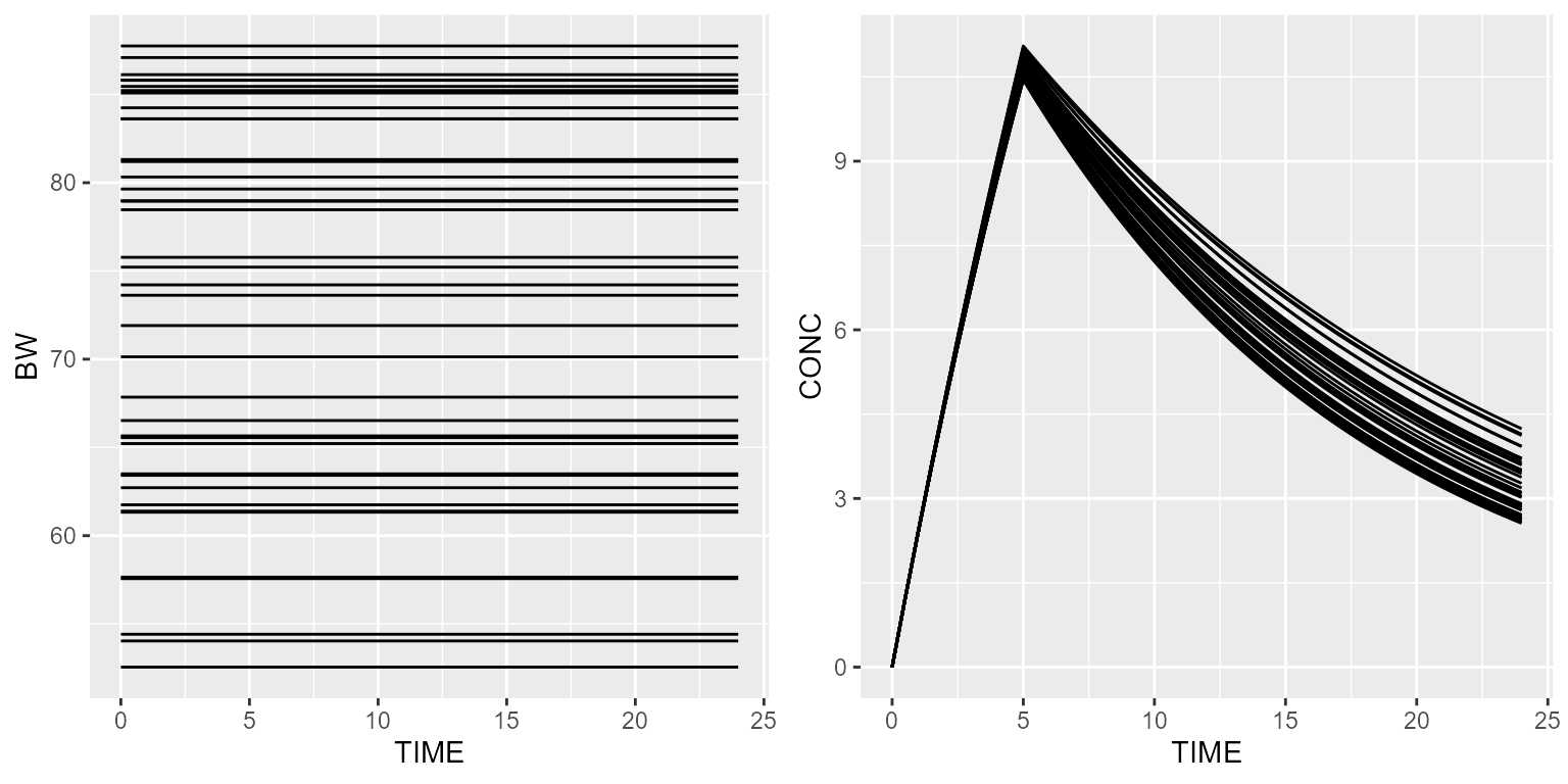
Normal distribution
Let’s say now that the body weight is a normal distribution. This can be implemented as follows:
ds <- dataset %>% setSubjects(40) %>%
  add(Covariate("BW", NormalDistribution(mean=70, sd=10)))
Simulated weights will then be sampled from a normal distribution with a mean of 70 and a standard deviation of 10.
results <- model %>% simulate(dataset=ds, outvars=c("CONC", "BW"), seed=1)
gridExtra::grid.arrange(spaghettiPlot(results, "BW"), spaghettiPlot(results, "CONC"), nrow=1)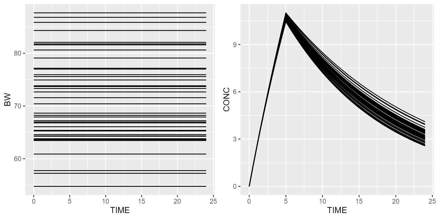
Log-normal distribution
Say now that the body weight is a log-normal distribution. This can be implemented as follows:
ds <- dataset %>% setSubjects(40) %>%
  add(Covariate("BW", LogNormalDistribution(meanlog=log(70), sdlog=0.2)))
Simulated weights will then be sampled from a log-normal distribution with a median of 70 and a coefficient of variation of 20%.
results <- model %>% simulate(dataset=ds, outvars=c("CONC", "BW"), seed=1)
gridExtra::grid.arrange(spaghettiPlot(results, "BW"), spaghettiPlot(results, "CONC"), nrow=1)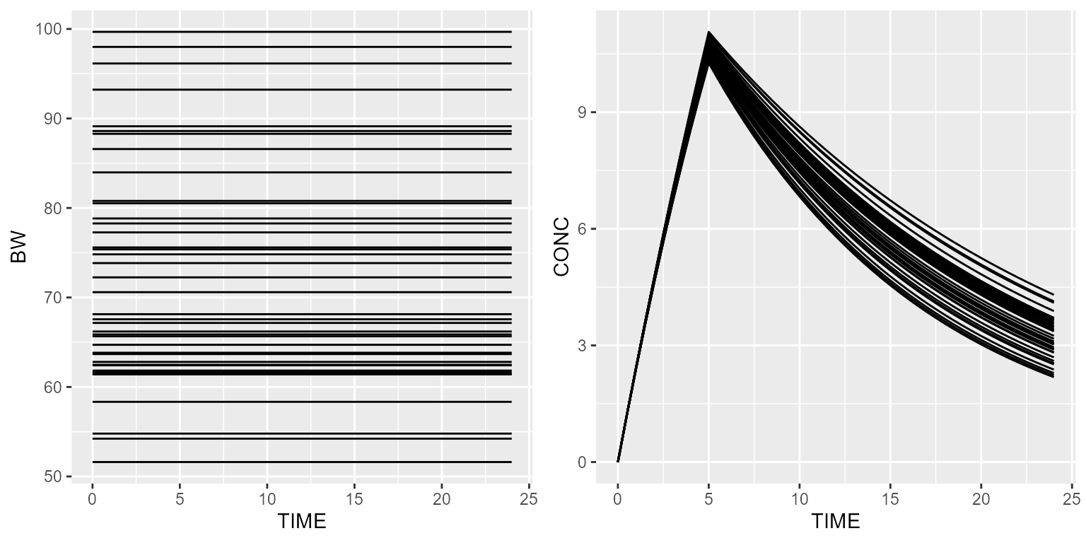
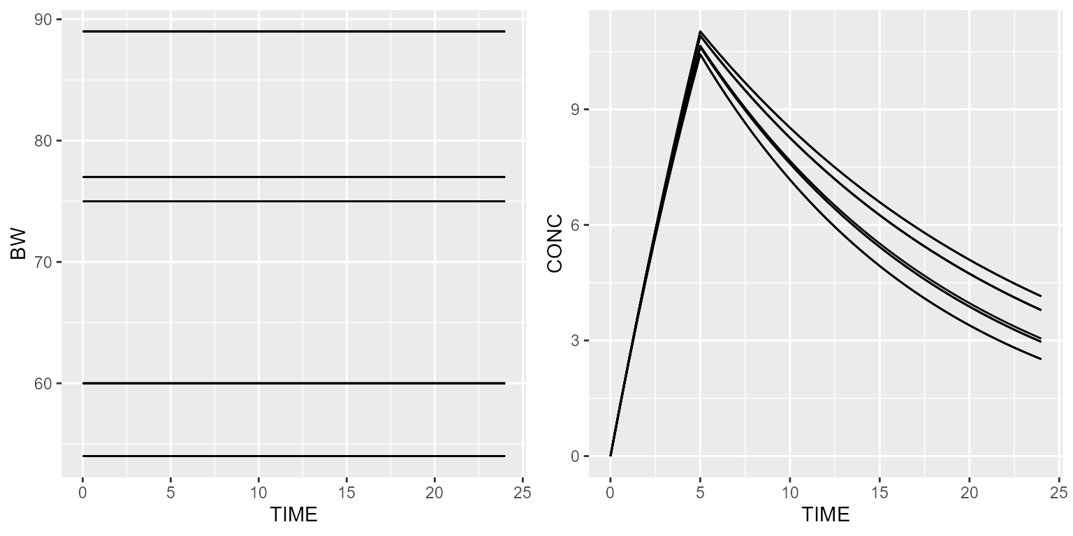
Bootstrap
Body weight can also be bootstrapped from a real dataset. Let’s create a fictive one:
bootstrap <- data.frame(ID=c(1,2,3,4,5), BW=c(89,54,60,75,77))
ds <- dataset %>% setSubjects(10) %>%
  add(Covariate("BW", BootstrapDistribution(data=bootstrap$BW, replacement=TRUE, random=TRUE)))
Simulated weights will then be sampled from a log-normal distribution with a median of 70 and a coefficient of variation of 20%.
results <- model %>% simulate(dataset=ds, outvars=c("CONC", "BW"), seed=2)
gridExtra::grid.arrange(spaghettiPlot(results, "BW"), spaghettiPlot(results, "CONC"), nrow=1)