Initial conditions • campsis

This vignette shows how initial conditions may be used in CAMPSIS.

Init central compartment

Assume the following 2-compartment model is used.

model <- model_suite$nonmem$advan3_trans4

We’d like to init the central compartment to a predefined value, e.g. 1000.
This can be achieved as follows.

model <- model %>% add(InitialCondition(compartment=1, rhs="1000"))

The resulting model has now a new block [INIT] which describes the initial condition:

model

## [MAIN]
## CL=THETA_CL*exp(ETA_CL)
## V1=THETA_V1*exp(ETA_V1)
## V2=THETA_V2*exp(ETA_V2)
## Q=THETA_Q*exp(ETA_Q)
## S1=V1
## 
## [ODE]
## d/dt(A_CENTRAL)=Q*A_PERIPHERAL/V2 + (-CL/V1 - Q/V1)*A_CENTRAL
## d/dt(A_PERIPHERAL)=-Q*A_PERIPHERAL/V2 + Q*A_CENTRAL/V1
## d/dt(A_OUTPUT)=CL*A_CENTRAL/V1
## F=A_CENTRAL/S1
## 
## [INIT]
## A_CENTRAL=1000
## 
## [ERROR]
## CONC=F
## CONC_ERR=CONC*(EPS_PROP + 1)
## 
## 
## THETA's:
##   name index value   fix
## 1   CL     1     5 FALSE
## 2   V1     2    80 FALSE
## 3   V2     3    20 FALSE
## 4    Q     4     4 FALSE
## OMEGA's:
##   name index index2 value   fix type
## 1   CL     1      1 0.025 FALSE  var
## 2   V1     2      2 0.025 FALSE  var
## 3   V2     3      3 0.025 FALSE  var
## 4    Q     4      4 0.025 FALSE  var
## SIGMA's:
##   name index index2 value   fix type
## 1 PROP     1      1 0.025 FALSE  var
## No variance-covariance matrix
## 
## Compartments:
## A_CENTRAL (CMT=1)
## A_PERIPHERAL (CMT=2)
## A_OUTPUT (CMT=3)

Let’s now create a dataset with observations-only.

ds <- Dataset(50) %>%
  add(Observations(times=seq(0,72, by=0.5)))

We can now simulate this model:

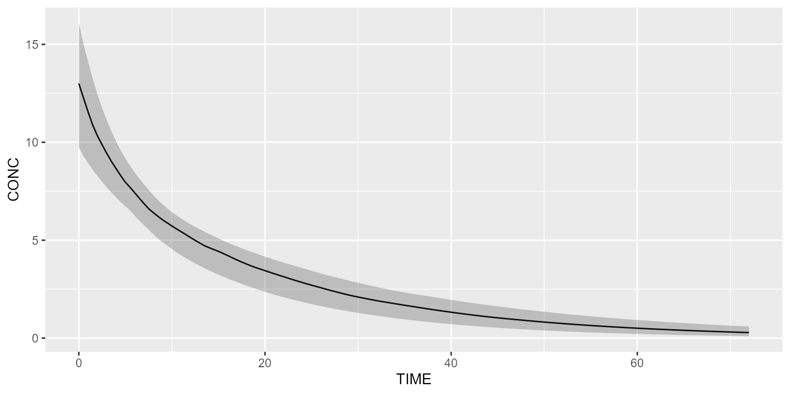
results <- model %>% simulate(dataset=ds, seed=1)
shadedPlot(results, "CONC")