There are 2 ways to implement a lag time in CAMPSIS:
- in the model: lag time is defined for each compartment
- in the dataset: lag time is defined for each bolus or infusion
In the first case, the simulation engine will take care of the lag time In the second case, CAMPSIS will adapt automatically the time of the dose(s)
Lag time implemented in model
Let’s use a 2-compartment model with absorption compartment to illustrate how this can be achieved.
model <- model_suite$nonmem$advan4_trans4For this example, we’re going to define a lag time ALAG1
for this absorption compartment.
First let’s create a new parameter ALAG1, log-normally
distributed with a median of 2 hours and 20% CV.
model <- model %>% add(Theta(name="ALAG1", value=2))
model <- model %>% add(Omega(name="ALAG1", value=20, type="cv%"))
Now, let’s add an equation to the drug model to define
ALAG1.
Finally, we need to tell CAMPSIS that ALAG1 corresponds
to a lag time.
Our persisted drug model would look like this:
model## [MAIN]
## KA=THETA_KA*exp(ETA_KA)
## CL=THETA_CL*exp(ETA_CL)
## V2=THETA_V2*exp(ETA_V2)
## V3=THETA_V3*exp(ETA_V3)
## Q=THETA_Q*exp(ETA_Q)
## S2=V2
## ALAG1=THETA_ALAG1*exp(ETA_ALAG1)
##
## [ODE]
## d/dt(A_DEPOT)=-KA*A_DEPOT
## d/dt(A_CENTRAL)=KA*A_DEPOT + Q*A_PERIPHERAL/V3 + (-CL/V2 - Q/V2)*A_CENTRAL
## d/dt(A_PERIPHERAL)=-Q*A_PERIPHERAL/V3 + Q*A_CENTRAL/V2
## d/dt(A_OUTPUT)=CL*A_CENTRAL/V2
## F=A_CENTRAL/S2
##
## [LAG]
## A_DEPOT=ALAG1
##
## [ERROR]
## CONC=F
## CONC_ERR=CONC*(EPS_PROP + 1)
##
##
## THETA's:
## name index value fix
## 1 KA 1 1 FALSE
## 2 CL 2 5 FALSE
## 3 V2 3 80 FALSE
## 4 V3 4 20 FALSE
## 5 Q 5 4 FALSE
## 6 ALAG1 6 2 FALSE
## OMEGA's:
## name index index2 value fix type
## 1 KA 1 1 0.025 FALSE var
## 2 CL 2 2 0.025 FALSE var
## 3 V2 3 3 0.025 FALSE var
## 4 V3 4 4 0.025 FALSE var
## 5 Q 5 5 0.025 FALSE var
## 6 ALAG1 6 6 20.000 FALSE cv%
## SIGMA's:
## name index index2 value fix type
## 1 PROP 1 1 0.025 FALSE var
## No variance-covariance matrix
##
## Compartments:
## A_DEPOT (CMT=1)
## A_CENTRAL (CMT=2)
## A_PERIPHERAL (CMT=3)
## A_OUTPUT (CMT=4)Now, let’s now give a simple bolus and simulate with and without
ALAG1.
ds1 <- Dataset(50) %>%
  add(Bolus(time=0, amount=1000)) %>%
  add(Observations(times=seq(0,24,by=0.5)))
results_alag <- model %>% simulate(dataset=ds1, seed=1)
results_no_alag <- model_suite$nonmem$advan4_trans4 %>% simulate(dataset=ds1, seed=1)
gridExtra::grid.arrange(shadedPlot(results_alag, "CONC"), shadedPlot(results_no_alag, "CONC"), nrow=1)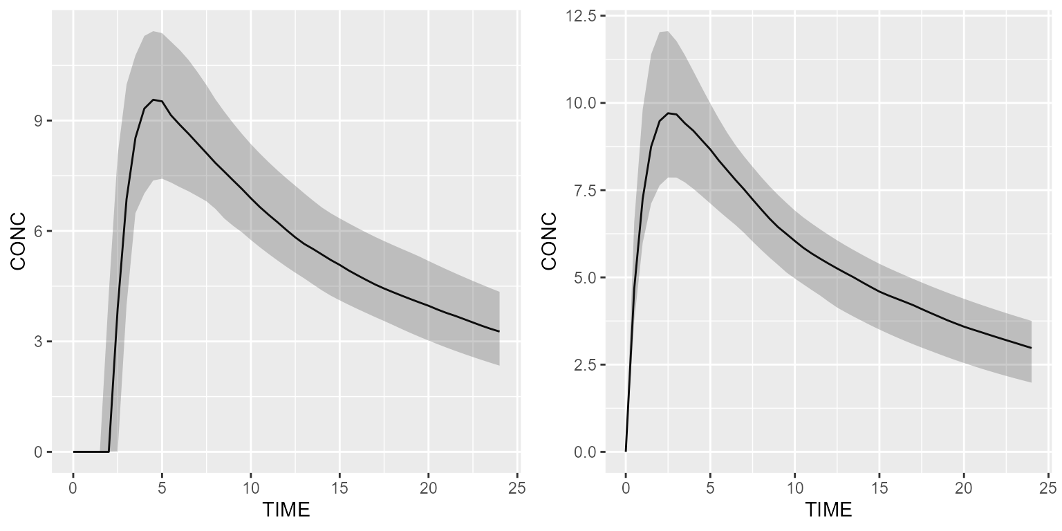
Lag time implemented in dataset
The same simulation can be performed by defining a lag time to the bolus in the dataset.
For this, we need to sample ALAG1 values. This can be
done as follows:
distribution <- ParameterDistribution(model=model, theta="ALAG1", omega="ALAG1") %>%
  sample(50L)
We can then pass the pre-sampled distribution.
ds2 <- Dataset(50) %>%
  add(Bolus(time=0, amount=1000, lag=distribution)) %>%
  add(Observations(times=seq(0,24,by=0.5)))
Here is an overview of the dataset in its table form if we filter on the doses:
## # A tibble: 6 × 9
## ID ARM TIME EVID MDV AMT CMT RATE DOSENO
## <dbl> <int> <dbl> <int> <int> <dbl> <chr> <dbl> <int>
## 1 1 0 1.77 1 1 1000 1 0 1
## 2 2 0 2.07 1 1 1000 1 0 1
## 3 3 0 1.69 1 1 1000 1 0 1
## 4 4 0 2.74 1 1 1000 1 0 1
## 5 5 0 2.13 1 1 1000 1 0 1
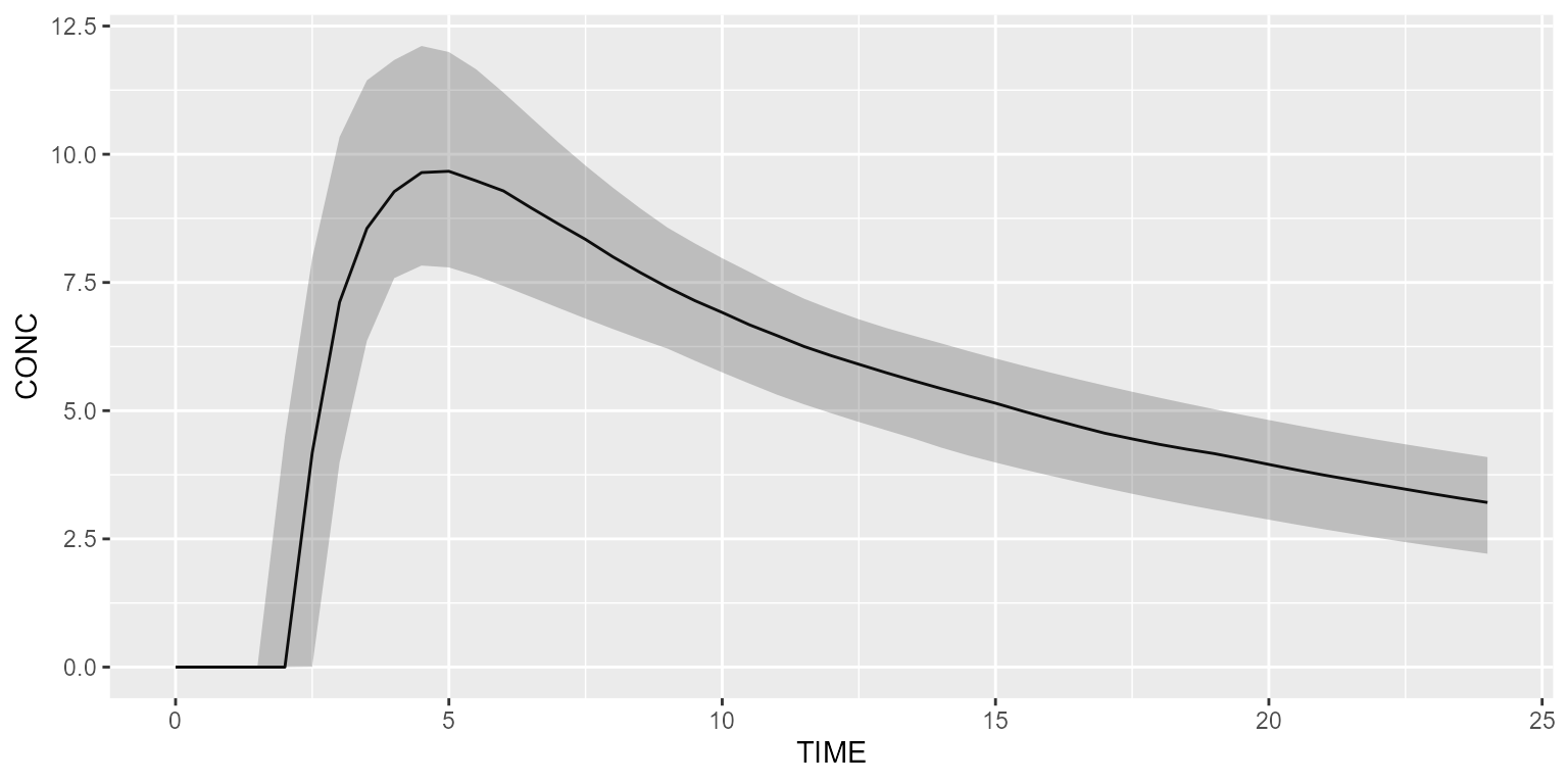
## 6 6 0 1.70 1 1 1000 1 0 1Let’s now simulate this dataset using the original model.
results_alag <- model_suite$nonmem$advan4_trans4 %>% simulate(dataset=ds2, seed=1)
shadedPlot(results_alag, "CONC")