Simple dose adaptations • campsis

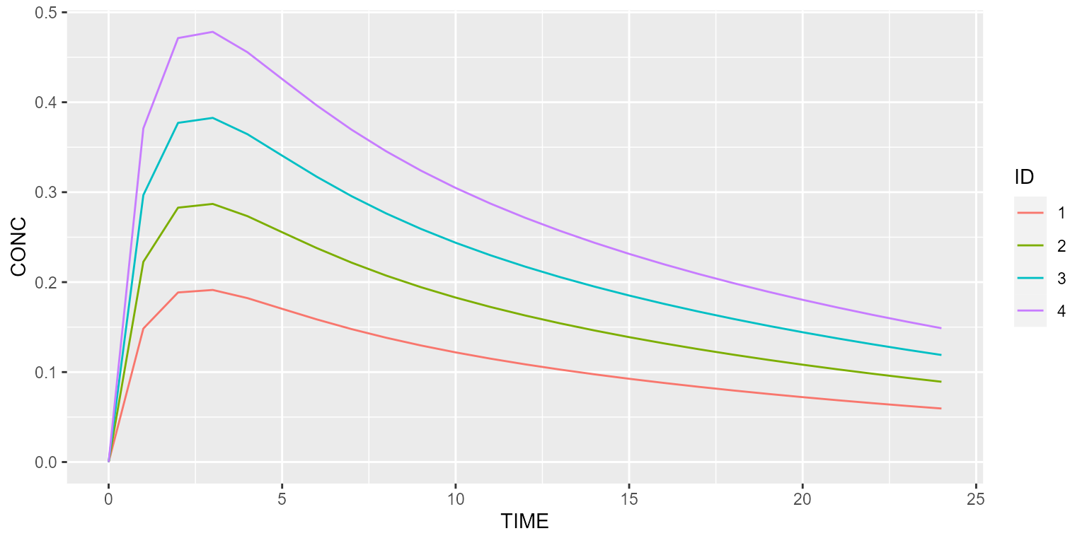
This vignette shows how simple dose adaptations can be implemented.

Adapt the dose based on a covariate

Assume that your drug needs to be dosed according to the subject’s weight, for instance 0.5 mg per kg. To illustrate this, let’s use our 2-compartment PK model with absorption compartment.

model <- model_suite$nonmem$advan4_trans4

We’re going to create a dataset with 4 individuals, weighing respectively 40, 60, 80 and 100 kg.

dataset <- Dataset(4) %>%
  add(Bolus(time=0, amount=0.5)) %>% # 0.5mg / kg
  add(Observations(times=0:24)) %>%
  add(Covariate("WT", c(40, 60, 80, 100)))

Our dataset is almost ready. We just have to define the dose adaptation formula. This is done as follows:

dataset <- dataset %>% add(DoseAdaptation("AMT*WT"))

Let’s simulate this simple dataset. In order to check that the dose adaptation formula was well applied, we set the argument dosing to TRUE. Dosing rows will then be returned.

results <- model %>% disable("IIV") %>% simulate(dataset=dataset, dosing=TRUE, seed=1)
spaghettiPlot(results, "CONC", "ID")

Let’s now have a look at the dosing information which is returned.

results %>% dosingOnly()

## # A tibble: 4 × 19
##      ID  EVID   CMT   AMT  TIME   ARM    KA    CL    V2    V3     Q    S2     F
##   <int> <int> <int> <dbl> <dbl> <dbl> <dbl> <dbl> <dbl> <dbl> <dbl> <dbl> <dbl>
## 1     1     1     1    20     0     0     1     5    80    20     4    80     0
## 2     2     1     1    30     0     0     1     5    80    20     4    80     0
## 3     3     1     1    40     0     0     1     5    80    20     4    80     0
## 4     4     1     1    50     0     0     1     5    80    20     4    80     0
## # ℹ 6 more variables: CONC <dbl>, CONC_ERR <dbl>, A_DEPOT <dbl>,
## #   A_CENTRAL <dbl>, A_PERIPHERAL <dbl>, A_OUTPUT <dbl>

This looks great! The respective amounts that were given are indeed 20, 30, 40 and 50 mg!