Time-varying covariates

This vignette shows how time-varying covariates can be implemented.

Body weight as a time varying covariate

As a demonstration example, let’s implement allometric scaling on the clearance and volume of a 1-compartment PK model:

model <- model_suite$nonmem$advan2_trans2
model <- model %>% replace(Equation("CL", "THETA_CL*exp(ETA_CL)*pow(BW/70, 0.75)"))
model <- model %>% replace(Equation("V", "THETA_V*exp(ETA_V)*BW/70"))

Assume our drug is given once a month and BW varies over time. A time-varying covariate can be added to the dataset as follows:

dataset <- Dataset(1) %>%
  add(Bolus(time=0, amount=1000)) %>%
  add(Observations(times=seq(0,30,by=0.1))) %>%
  add(TimeVaryingCovariate("BW", data.frame(TIME=c(0,7,14,21), VALUE=c(80,75,70,65))))

The typical profile can be simulated in the following way:

results <- model %>% disable("IIV") %>% simulate(dataset, seed=1, outvars="BW")
gridExtra::grid.arrange(spaghettiPlot(results, "CONC"),
                        spaghettiPlot(results, "BW"), ncol=1)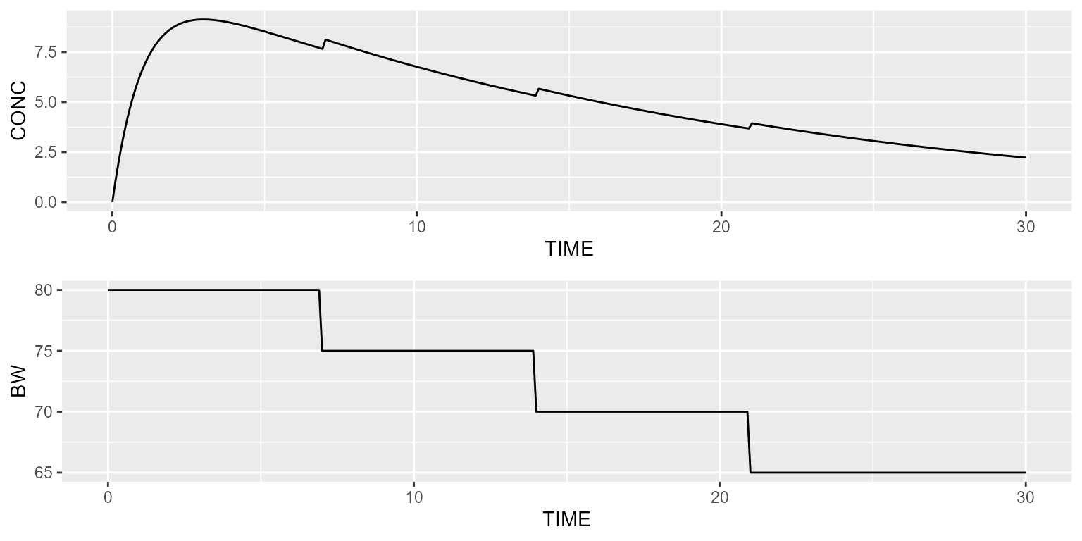

Let’s now compare this profile with another typical individual having a constant body weight of 70 kg:

scenarios <- Scenarios() %>%
  add(Scenario("BW as time-varying covarite")) %>%
  add(Scenario("Fixed BW", dataset=~.x %>% replace(Covariate("BW", 70))))

results <- model %>% disable("IIV") %>% simulate(dataset, seed=1, outvars="BW", scenarios=scenarios)
gridExtra::grid.arrange(spaghettiPlot(results, "CONC", "SCENARIO"),
                        spaghettiPlot(results, "BW", "SCENARIO"), ncol=1)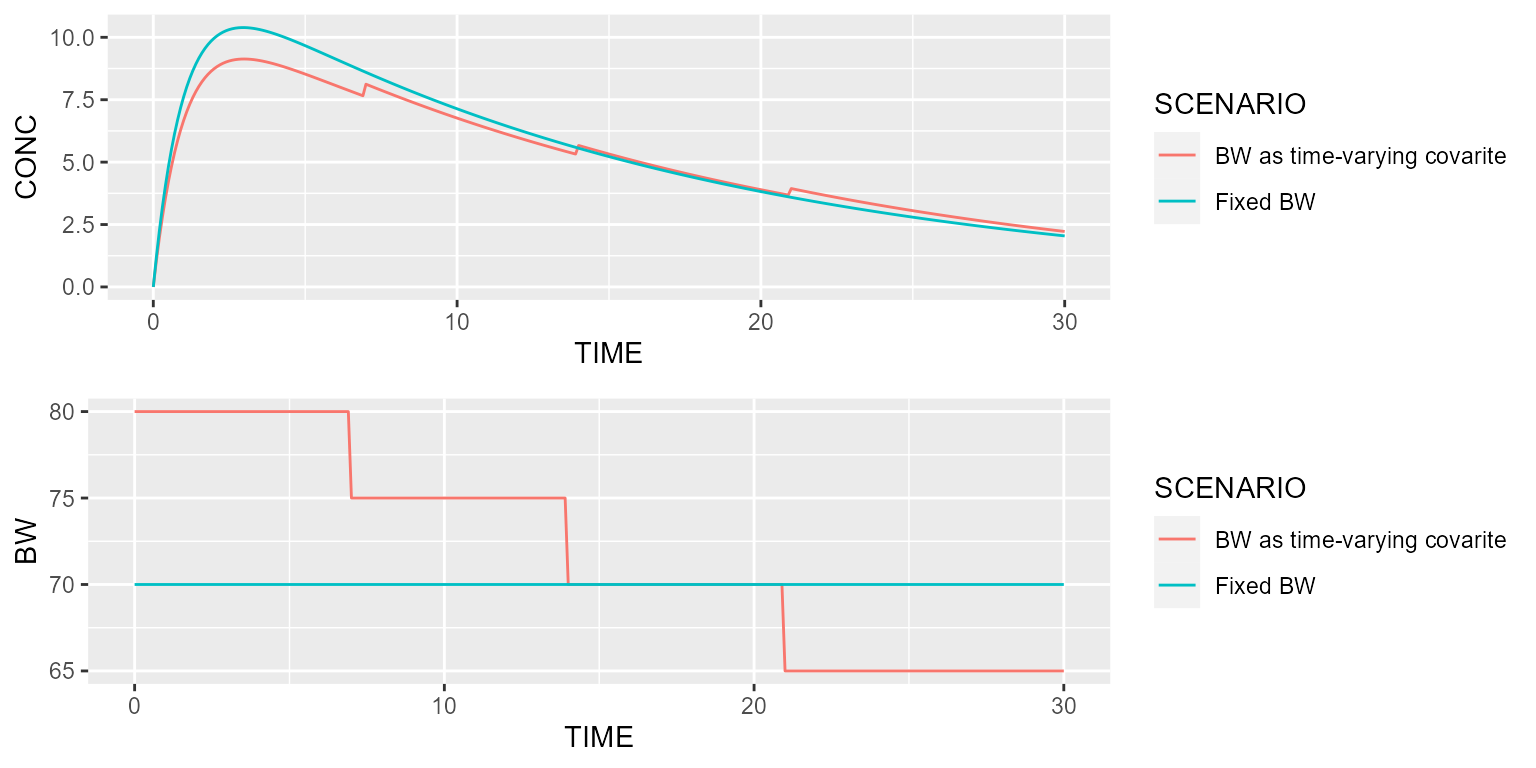

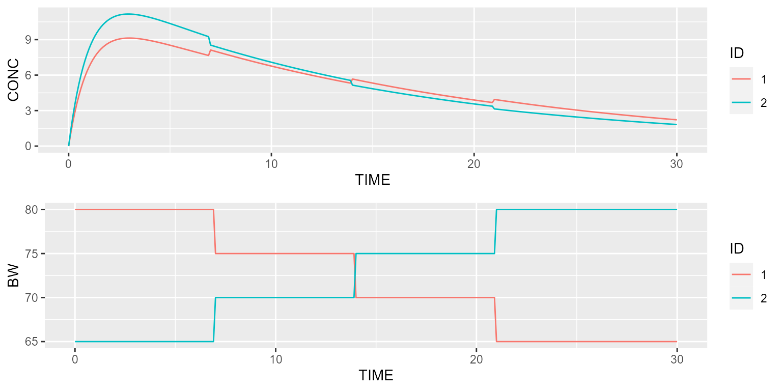
Finally, time-varying covariates can also be individualized by specifying an ID column:

dataset <- Dataset(2) %>%
  add(Bolus(time=0, amount=1000)) %>%
  add(Observations(times=seq(0,30,by=0.1))) %>%
  add(TimeVaryingCovariate("BW", data.frame(ID=c(rep(1, 4), rep(2, 4)),
                                            TIME=c(0,7,14,21, 0,7,14,21),
                                            VALUE=c(80,75,70,65, 65,70,75,80))))
results <- model %>% disable("IIV") %>% simulate(dataset, seed=1, outvars="BW")
gridExtra::grid.arrange(spaghettiPlot(results, "CONC", "ID"),
                        spaghettiPlot(results, "BW", "ID"), ncol=1)