Replicate your study

This vignette shows how a simulation can be replicated.

Simulate uncertainty on percentiles

Assume the following model is used. This model is a 2-compartment model without absorption compartment which has been fitted on some data.

model <- model_suite$testing$other$my_model1

It contains a variance-covariance matrix with the uncertainty on all the estimated parameters.

model

## [MAIN]
## CL=THETA_CL*exp(ETA_CL)
## V1=THETA_V1*exp(ETA_V1)
## V2=THETA_V2
## Q=THETA_Q
## S1=V1
## 
## [ODE]
## d/dt(A_CENTRAL)=Q*A_PERIPHERAL/V2 + (-CL/V1 - Q/V1)*A_CENTRAL
## d/dt(A_PERIPHERAL)=-Q*A_PERIPHERAL/V2 + Q*A_CENTRAL/V1
## d/dt(A_OUTPUT)=CL*A_CENTRAL/V1
## F=A_CENTRAL/S1
## 
## [DURATION]
## A_CENTRAL=5
## 
## [ERROR]
## CP=F
## OBS_CP=CP*(EPS_PROP + 1)
## Y=OBS_CP
## 
## 
## THETA's:
##   name index    value   fix        se      rse%
## 1   CL     1  4.76756 FALSE 0.1163899  2.441288
## 2   V1     2 82.64090 FALSE 1.9256999  2.330202
## 3   V2     3 19.53960 FALSE 1.5382328  7.872386
## 4    Q     4  3.81451 FALSE 0.4726151 12.389929
## OMEGA's:
##   name index index2     value   fix type          se     rse%
## 1   CL     1      1 0.0222955 FALSE  var 0.004867504 21.83178
## 2   V1     2      2 0.0182225 FALSE  var 0.005172881 28.38733
## SIGMA's:
##   name index index2     value   fix type           se    rse%
## 1 PROP     1      1 0.0244587 FALSE  var 0.0008126574 3.32257
## Variance-covariance matrix available (see ?getVarCov)
## 
## Compartments:
## A_CENTRAL (CMT=1)
## A_PERIPHERAL (CMT=2)
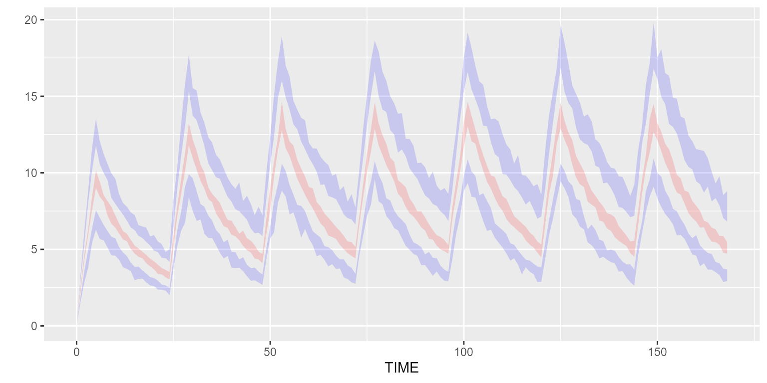
## A_OUTPUT (CMT=3)

We are interested to see the uncertainty on the simulated concentration percentiles over time. Let’s mimic the protocol that was implemented in the study.

ds <- Dataset(50) %>%
  add(Infusion(time=(0:6)*24, amount=1000, compartment=1)) %>%
  add(Observations(times=seq(0, 7*24)))

Let’s now simulate this model with parameter uncertainty.
Argument replicates specifies how many times the simulation is replicated.
Argument outfun is a function that is going to be called after each simulation on the output data frame.

results <- model %>% simulate(dataset=ds, replicates=10, outfun=~PI(.x, output="Y"), seed=1)
results %>% head()

## # A tibble: 6 × 4
## # Groups:   TIME [2]
##   replicate  TIME metric value
##       <int> <dbl> <chr>  <dbl>
## 1         1     0 med     0   
## 2         1     0 low     0   
## 3         1     0 up      0   
## 4         1     1 med     2.33
## 5         1     1 low     1.64
## 6         1     1 up      3.03

Function vpcPlot allows to quickly visualize such results.

vpcPlot(results)